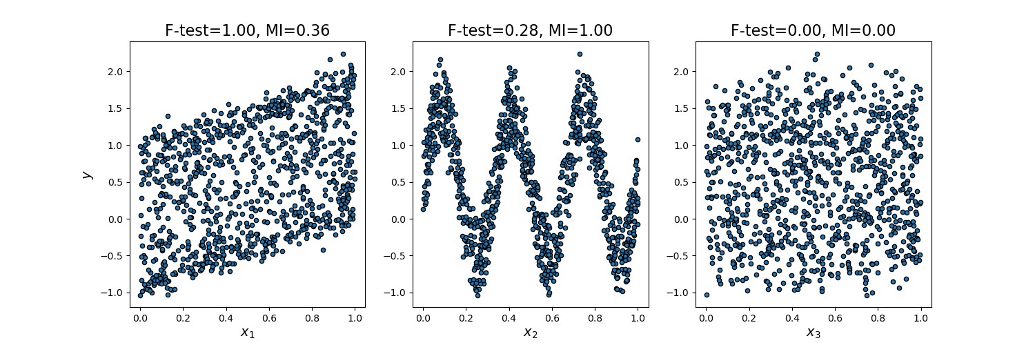
This example illustrates the differences between univariate F-test statistics and mutual information.
We consider 3 features x_1, x_2, x_3 distributed uniformly over [0, 1], the target depends on them as follows:
y = x_1 + sin(6 * pi * x_2) + 0.1 * N(0, 1), that is the third features is completely irrelevant.
The code below plots the dependency of y against individual x_i and normalized values of univariate F-tests statistics and mutual information.
As F-test captures only linear dependency, it rates x_1 as the most discriminative feature. On the other hand, mutual information can capture any kind of dependency between variables and it rates x_2 as the most discriminative feature, which probably agrees better with our intuitive perception for this example. Both methods correctly marks x_3 as irrelevant.
print(__doc__)

import numpy as np
import matplotlib.pyplot as plt
from sklearn.feature_selection import f_regression, mutual_info_regression

np.random.seed(0)
X = np.random.rand(1000, 3)
y = X[:, 0] + np.sin(6 * np.pi * X[:, 1]) + 0.1 * np.random.randn(1000)

f_test, _ = f_regression(X, y)
f_test /= np.max(f_test)

mi = mutual_info_regression(X, y)
mi /= np.max(mi)

plt.figure(figsize=(15, 5))
for i in range(3):
    plt.subplot(1, 3, i + 1)
    plt.scatter(X[:, i], y)
    plt.xlabel("$x_{}$".format(i + 1), fontsize=14)
    if i == 0:
        plt.ylabel("$y$", fontsize=14)
    plt.title("F-test={:.2f}, MI={:.2f}".format(f_test[i], mi[i]),
              fontsize=16)
plt.show()
Total running time of the script: (0 minutes 0.221 seconds)
plot_f_test_vs_mi.py
plot_f_test_vs_mi.ipynb
Please login to continue.