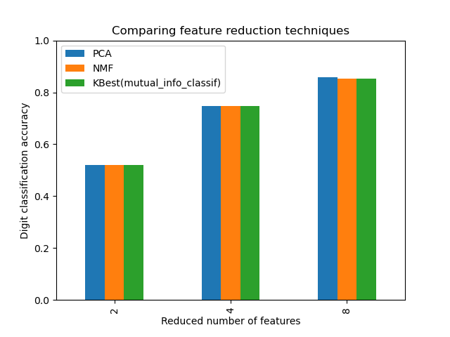
Selecting dimensionality reduction with Pipeline and GridSearchCV

This example constructs a pipeline that does dimensionality reduction followed by prediction with a support vector classifier. It demonstrates the use of GridSearchCV and Pipeline to optimize over different classes of estimators in a single CV run ? unsupervised PCA and NMF dimensionality reductions are compared to univariate feature selection during the grid search.

../_images/sphx_glr_plot_compare_reduction_001.png

# Authors: Robert McGibbon, Joel Nothman
 
from __future__ import print_function, division
 
import numpy as np
import matplotlib.pyplot as plt
from sklearn.datasets import load_digits
from sklearn.model_selection import GridSearchCV
from sklearn.pipeline import Pipeline
from sklearn.svm import LinearSVC
from sklearn.decomposition import PCA, NMF
from sklearn.feature_selection import SelectKBest, chi2
 
print(__doc__)
 
pipe = Pipeline([
    ('reduce_dim', PCA()),
    ('classify', LinearSVC())
])
 
N_FEATURES_OPTIONS = [2, 4, 8]
C_OPTIONS = [1, 10, 100, 1000]
param_grid = [
    {
        'reduce_dim': [PCA(iterated_power=7), NMF()],
        'reduce_dim__n_components': N_FEATURES_OPTIONS,
        'classify__C': C_OPTIONS
    },
    {
        'reduce_dim': [SelectKBest(chi2)],
        'reduce_dim__k': N_FEATURES_OPTIONS,
        'classify__C': C_OPTIONS
    },
]
reducer_labels = ['PCA', 'NMF', 'KBest(chi2)']
 
grid = GridSearchCV(pipe, cv=3, n_jobs=2, param_grid=param_grid)
digits = load_digits()
grid.fit(digits.data, digits.target)
 
mean_scores = np.array(grid.cv_results_['mean_test_score'])
# scores are in the order of param_grid iteration, which is alphabetical
mean_scores = mean_scores.reshape(len(C_OPTIONS), -1, len(N_FEATURES_OPTIONS))
# select score for best C
mean_scores = mean_scores.max(axis=0)
bar_offsets = (np.arange(len(N_FEATURES_OPTIONS)) *
               (len(reducer_labels) + 1) + .5)
 
plt.figure()
COLORS = 'bgrcmyk'
for i, (label, reducer_scores) in enumerate(zip(reducer_labels, mean_scores)):
    plt.bar(bar_offsets + i, reducer_scores, label=label, color=COLORS[i])
 
plt.title("Comparing feature reduction techniques")
plt.xlabel('Reduced number of features')
plt.xticks(bar_offsets + len(reducer_labels) / 2, N_FEATURES_OPTIONS)
plt.ylabel('Digit classification accuracy')
plt.ylim((0, 1))
plt.legend(loc='upper left')
plt.show()

Total running time of the script: (0 minutes 39.990 seconds)

Download Python source code: plot_compare_reduction.py

Download IPython notebook: plot_compare_reduction.ipynb

Links:

http://scikit-learn.org/stable/auto_examples/plot_compare_reduction.html

doc_scikit_learn

2025-01-10 15:47:30

Comments