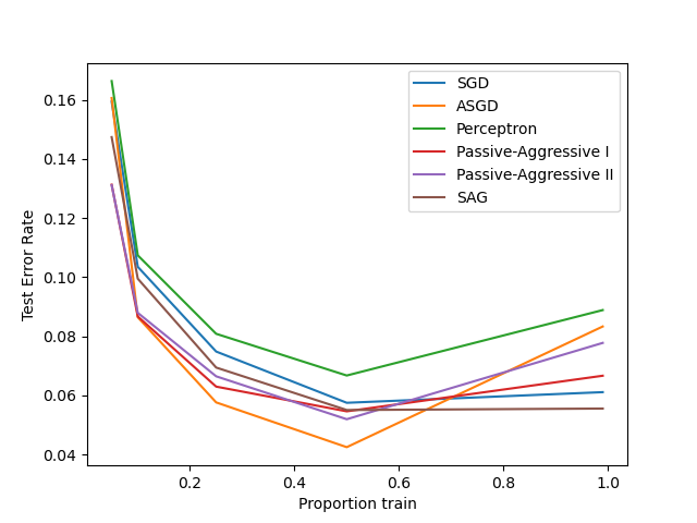
An example showing how different online solvers perform on the hand-written digits dataset.
Out:
  training SGD
training ASGD
training Perceptron
training Passive-Aggressive I
training Passive-Aggressive II
training SAG
# Author: Rob Zinkov <rob at zinkov dot com>
# License: BSD 3 clause

import numpy as np
import matplotlib.pyplot as plt
from sklearn import datasets

from sklearn.model_selection import train_test_split
from sklearn.linear_model import SGDClassifier, Perceptron
from sklearn.linear_model import PassiveAggressiveClassifier
from sklearn.linear_model import LogisticRegression

heldout = [0.95, 0.90, 0.75, 0.50, 0.01]
rounds = 20
digits = datasets.load_digits()
X, y = digits.data, digits.target

classifiers = [
    ("SGD", SGDClassifier()),
    ("ASGD", SGDClassifier(average=True)),
    ("Perceptron", Perceptron()),
    ("Passive-Aggressive I", PassiveAggressiveClassifier(loss='hinge',
                                                         C=1.0)),
    ("Passive-Aggressive II", PassiveAggressiveClassifier(loss='squared_hinge',
                                                          C=1.0)),
    ("SAG", LogisticRegression(solver='sag', tol=1e-1, C=1.e4 / X.shape[0]))
]

xx = 1. - np.array(heldout)

for name, clf in classifiers:
    print("training %s" % name)
    rng = np.random.RandomState(42)
    yy = []
    for i in heldout:
        yy_ = []
        for r in range(rounds):
            X_train, X_test, y_train, y_test = \
                train_test_split(X, y, test_size=i, random_state=rng)
            clf.fit(X_train, y_train)
            y_pred = clf.predict(X_test)
            yy_.append(1 - np.mean(y_pred == y_test))
        yy.append(np.mean(yy_))
    plt.plot(xx, yy, label=name)

plt.legend(loc="upper right")
plt.xlabel("Proportion train")
plt.ylabel("Test Error Rate")
plt.show()
Total running time of the script: (0 minutes 13.767 seconds)
Download Python source code:
plot_sgd_comparison.py
Download IPython notebook:
plot_sgd_comparison.ipynb
Please login to continue.