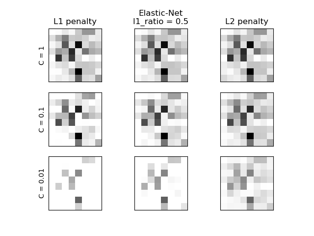
Comparison of the sparsity (percentage of zero coefficients) of solutions when L1 and L2 penalty are used for different values of C. We can see that large values of C give more freedom to the model. Conversely, smaller values of C constrain the model more. In the L1 penalty case, this leads to sparser solutions.
We classify 8x8 images of digits into two classes: 0-4 against 5-9. The visualization shows coefficients of the models for varying C.
Out:
  C=100.00
Sparsity with L1 penalty: 6.25%
score with L1 penalty: 0.9104
Sparsity with L2 penalty: 4.69%
score with L2 penalty: 0.9098
C=1.00
Sparsity with L1 penalty: 10.94%
score with L1 penalty: 0.9104
Sparsity with L2 penalty: 4.69%
score with L2 penalty: 0.9093
C=0.01
Sparsity with L1 penalty: 85.94%
score with L1 penalty: 0.8614
Sparsity with L2 penalty: 4.69%
score with L2 penalty: 0.8915
print(__doc__)

# Authors: Alexandre Gramfort <alexandre.gramfort@inria.fr>
#          Mathieu Blondel <mathieu@mblondel.org>
#          Andreas Mueller <amueller@ais.uni-bonn.de>
# License: BSD 3 clause

import numpy as np
import matplotlib.pyplot as plt

from sklearn.linear_model import LogisticRegression
from sklearn import datasets
from sklearn.preprocessing import StandardScaler

digits = datasets.load_digits()

X, y = digits.data, digits.target
X = StandardScaler().fit_transform(X)

# classify small against large digits
y = (y > 4).astype(np.int)


# Set regularization parameter
for i, C in enumerate((100, 1, 0.01)):
    # turn down tolerance for short training time
    clf_l1_LR = LogisticRegression(C=C, penalty='l1', tol=0.01)
    clf_l2_LR = LogisticRegression(C=C, penalty='l2', tol=0.01)
    clf_l1_LR.fit(X, y)
    clf_l2_LR.fit(X, y)

    coef_l1_LR = clf_l1_LR.coef_.ravel()
    coef_l2_LR = clf_l2_LR.coef_.ravel()

    # coef_l1_LR contains zeros due to the
    # L1 sparsity inducing norm

    sparsity_l1_LR = np.mean(coef_l1_LR == 0) * 100
    sparsity_l2_LR = np.mean(coef_l2_LR == 0) * 100

    print("C=%.2f" % C)
    print("Sparsity with L1 penalty: %.2f%%" % sparsity_l1_LR)
    print("score with L1 penalty: %.4f" % clf_l1_LR.score(X, y))
    print("Sparsity with L2 penalty: %.2f%%" % sparsity_l2_LR)
    print("score with L2 penalty: %.4f" % clf_l2_LR.score(X, y))

    l1_plot = plt.subplot(3, 2, 2 * i + 1)
    l2_plot = plt.subplot(3, 2, 2 * (i + 1))
    if i == 0:
        l1_plot.set_title("L1 penalty")
        l2_plot.set_title("L2 penalty")

    l1_plot.imshow(np.abs(coef_l1_LR.reshape(8, 8)), interpolation='nearest',
                   cmap='binary', vmax=1, vmin=0)
    l2_plot.imshow(np.abs(coef_l2_LR.reshape(8, 8)), interpolation='nearest',
                   cmap='binary', vmax=1, vmin=0)
    plt.text(-8, 3, "C = %.2f" % C)

    l1_plot.set_xticks(())
    l1_plot.set_yticks(())
    l2_plot.set_xticks(())
    l2_plot.set_yticks(())

plt.show()
Total running time of the script: (0 minutes 0.688 seconds)
Download Python source code:
plot_logistic_l1_l2_sparsity.py
Download IPython notebook:
plot_logistic_l1_l2_sparsity.ipynb
Please login to continue.