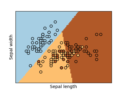
Show below is a logistic-regression classifiers decision boundaries on the iris dataset. The datapoints are colored according to their labels.
print(__doc__)


# Code source: Ga Varoquaux
# Modified for documentation by Jaques Grobler
# License: BSD 3 clause

import numpy as np
import matplotlib.pyplot as plt
from sklearn import linear_model, datasets

# import some data to play with
iris = datasets.load_iris()
X = iris.data[:, :2]  # we only take the first two features.
Y = iris.target

h = .02  # step size in the mesh

logreg = linear_model.LogisticRegression(C=1e5)

# we create an instance of Neighbours Classifier and fit the data.
logreg.fit(X, Y)

# Plot the decision boundary. For that, we will assign a color to each
# point in the mesh [x_min, x_max]x[y_min, y_max].
x_min, x_max = X[:, 0].min() - .5, X[:, 0].max() + .5
y_min, y_max = X[:, 1].min() - .5, X[:, 1].max() + .5
xx, yy = np.meshgrid(np.arange(x_min, x_max, h), np.arange(y_min, y_max, h))
Z = logreg.predict(np.c_[xx.ravel(), yy.ravel()])

# Put the result into a color plot
Z = Z.reshape(xx.shape)
plt.figure(1, figsize=(4, 3))
plt.pcolormesh(xx, yy, Z, cmap=plt.cm.Paired)

# Plot also the training points
plt.scatter(X[:, 0], X[:, 1], c=Y, edgecolors='k', cmap=plt.cm.Paired)
plt.xlabel('Sepal length')
plt.ylabel('Sepal width')

plt.xlim(xx.min(), xx.max())
plt.ylim(yy.min(), yy.max())
plt.xticks(())
plt.yticks(())

plt.show()
Total running time of the script: (0 minutes 0.087 seconds)
Download Python source code:
plot_iris_logistic.py
Download IPython notebook:
plot_iris_logistic.ipynb
Please login to continue.