Swiss Roll reduction with LLE

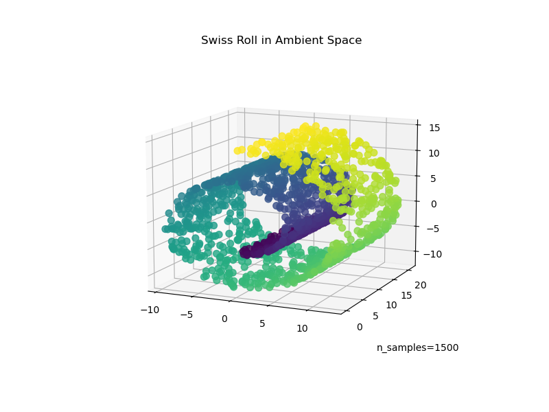
An illustration of Swiss Roll reduction with locally linear embedding

../../_images/sphx_glr_plot_swissroll_001.png

Out:

  Computing LLE embedding
Done. Reconstruction error: 9.45487e-08

# Author: Fabian Pedregosa -- <fabian.pedregosa@inria.fr>
# License: BSD 3 clause (C) INRIA 2011
 
print(__doc__)
 
import matplotlib.pyplot as plt
 
# This import is needed to modify the way figure behaves
from mpl_toolkits.mplot3d import Axes3D
Axes3D
 
#----------------------------------------------------------------------
# Locally linear embedding of the swiss roll
 
from sklearn import manifold, datasets
X, color = datasets.samples_generator.make_swiss_roll(n_samples=1500)
 
print("Computing LLE embedding")
X_r, err = manifold.locally_linear_embedding(X, n_neighbors=12,
                                             n_components=2)
print("Done. Reconstruction error: %g" % err)
 
#----------------------------------------------------------------------
# Plot result
 
fig = plt.figure()
try:
    # compatibility matplotlib < 1.0
    ax = fig.add_subplot(211, projection='3d')
    ax.scatter(X[:, 0], X[:, 1], X[:, 2], c=color, cmap=plt.cm.Spectral)
except:
    ax = fig.add_subplot(211)
    ax.scatter(X[:, 0], X[:, 2], c=color, cmap=plt.cm.Spectral)
 
ax.set_title("Original data")
ax = fig.add_subplot(212)
ax.scatter(X_r[:, 0], X_r[:, 1], c=color, cmap=plt.cm.Spectral)
plt.axis('tight')
plt.xticks([]), plt.yticks([])
plt.title('Projected data')
plt.show()

Total running time of the script: (0 minutes 0.412 seconds)

Download Python source code: plot_swissroll.py

Download IPython notebook: plot_swissroll.ipynb

Links:

http://scikit-learn.org/stable/auto_examples/manifold/plot_swissroll.html

doc_scikit_learn

2025-01-10 15:47:30

Comments