Label Propagation digits

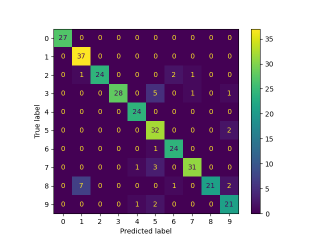
This example demonstrates the power of semisupervised learning by training a Label Spreading model to classify handwritten digits with sets of very few labels.

The handwritten digit dataset has 1797 total points. The model will be trained using all points, but only 30 will be labeled. Results in the form of a confusion matrix and a series of metrics over each class will be very good.

At the end, the top 10 most uncertain predictions will be shown.

print(__doc__)
 
# Authors: Clay Woolam <clay@woolam.org>
# License: BSD
 
import numpy as np
import matplotlib.pyplot as plt
 
from scipy import stats
 
from sklearn import datasets
from sklearn.semi_supervised import label_propagation
 
from sklearn.metrics import confusion_matrix, classification_report
 
digits = datasets.load_digits()
rng = np.random.RandomState(0)
indices = np.arange(len(digits.data))
rng.shuffle(indices)
 
X = digits.data[indices[:330]]
y = digits.target[indices[:330]]
images = digits.images[indices[:330]]
 
n_total_samples = len(y)
n_labeled_points = 30
 
indices = np.arange(n_total_samples)
 
unlabeled_set = indices[n_labeled_points:]
 
# shuffle everything around
y_train = np.copy(y)
y_train[unlabeled_set] = -1

Learn with LabelSpreading

lp_model = label_propagation.LabelSpreading(gamma=0.25, max_iter=5)
lp_model.fit(X, y_train)
predicted_labels = lp_model.transduction_[unlabeled_set]
true_labels = y[unlabeled_set]
 
cm = confusion_matrix(true_labels, predicted_labels, labels=lp_model.classes_)
 
print("Label Spreading model: %d labeled & %d unlabeled points (%d total)" %
      (n_labeled_points, n_total_samples - n_labeled_points, n_total_samples))
 
print(classification_report(true_labels, predicted_labels))
 
print("Confusion matrix")
print(cm)
 
# calculate uncertainty values for each transduced distribution
pred_entropies = stats.distributions.entropy(lp_model.label_distributions_.T)
 
# pick the top 10 most uncertain labels
uncertainty_index = np.argsort(pred_entropies)[-10:]

Out:

  Label Spreading model: 30 labeled & 300 unlabeled points (330 total)
             precision    recall  f1-score   support
 
          0       1.00      1.00      1.00        23
          1       0.58      0.54      0.56        28
          2       0.96      0.93      0.95        29
          3       0.00      0.00      0.00        28
          4       0.91      0.80      0.85        25
          5       0.96      0.79      0.87        33
          6       0.97      0.97      0.97        36
          7       0.89      1.00      0.94        34
          8       0.48      0.83      0.61        29
          9       0.54      0.77      0.64        35
 
avg / total       0.73      0.77      0.74       300
 
Confusion matrix
[[23  0  0  0  0  0  0  0  0]
 [ 0 15  1  0  0  1  0 11  0]
 [ 0  0 27  0  0  0  2  0  0]
 [ 0  5  0 20  0  0  0  0  0]
 [ 0  0  0  0 26  0  0  1  6]
 [ 0  1  0  0  0 35  0  0  0]
 [ 0  0  0  0  0  0 34  0  0]
 [ 0  5  0  0  0  0  0 24  0]
 [ 0  0  0  2  1  0  2  3 27]]

plot

f = plt.figure(figsize=(7, 5))
for index, image_index in enumerate(uncertainty_index):
    image = images[image_index]
 
    sub = f.add_subplot(2, 5, index + 1)
    sub.imshow(image, cmap=plt.cm.gray_r)
    plt.xticks([])
    plt.yticks([])
    sub.set_title('predict: %i\ntrue: %i' % (
        lp_model.transduction_[image_index], y[image_index]))
 
f.suptitle('Learning with small amount of labeled data')
plt.show()

../../_images/sphx_glr_plot_label_propagation_digits_001.png

Total running time of the script: (0 minutes 0.954 seconds)

Download Python source code: plot_label_propagation_digits.py

Download IPython notebook: plot_label_propagation_digits.ipynb

Links:

http://scikit-learn.org/stable/auto_examples/semi_supervised/plot_label_propagation_digits.html

doc_scikit_learn

2025-01-10 15:47:30

Comments