SVM-Kernels

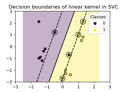
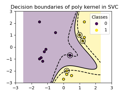
Three different types of SVM-Kernels are displayed below. The polynomial and RBF are especially useful when the data-points are not linearly separable.

print(__doc__)
 
 
# Code source: Ga Varoquaux
# License: BSD 3 clause
 
import numpy as np
import matplotlib.pyplot as plt
from sklearn import svm
 
 
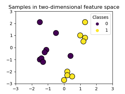
# Our dataset and targets
X = np.c_[(.4, -.7),
          (-1.5, -1),
          (-1.4, -.9),
          (-1.3, -1.2),
          (-1.1, -.2),
          (-1.2, -.4),
          (-.5, 1.2),
          (-1.5, 2.1),
          (1, 1),
          # --
          (1.3, .8),
          (1.2, .5),
          (.2, -2),
          (.5, -2.4),
          (.2, -2.3),
          (0, -2.7),
          (1.3, 2.1)].T
Y = [0] * 8 + [1] * 8
 
# figure number
fignum = 1
 
# fit the model
for kernel in ('linear', 'poly', 'rbf'):
    clf = svm.SVC(kernel=kernel, gamma=2)
    clf.fit(X, Y)
 
    # plot the line, the points, and the nearest vectors to the plane
    plt.figure(fignum, figsize=(4, 3))
    plt.clf()
 
    plt.scatter(clf.support_vectors_[:, 0], clf.support_vectors_[:, 1], s=80,
                facecolors='none', zorder=10)
    plt.scatter(X[:, 0], X[:, 1], c=Y, zorder=10, cmap=plt.cm.Paired)
 
    plt.axis('tight')
    x_min = -3
    x_max = 3
    y_min = -3
    y_max = 3
 
    XX, YY = np.mgrid[x_min:x_max:200j, y_min:y_max:200j]
    Z = clf.decision_function(np.c_[XX.ravel(), YY.ravel()])
 
    # Put the result into a color plot
    Z = Z.reshape(XX.shape)
    plt.figure(fignum, figsize=(4, 3))
    plt.pcolormesh(XX, YY, Z > 0, cmap=plt.cm.Paired)
    plt.contour(XX, YY, Z, colors=['k', 'k', 'k'], linestyles=['--', '-', '--'],
                levels=[-.5, 0, .5])
 
    plt.xlim(x_min, x_max)
    plt.ylim(y_min, y_max)
 
    plt.xticks(())
    plt.yticks(())
    fignum = fignum + 1
plt.show()

Total running time of the script: (0 minutes 0.305 seconds)

Download Python source code: plot_svm_kernels.py

Download IPython notebook: plot_svm_kernels.ipynb

Links:

http://scikit-learn.org/stable/auto_examples/svm/plot_svm_kernels.html

doc_scikit_learn

2025-01-10 15:47:30

Comments