SVM with custom kernel

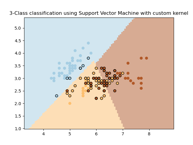
Simple usage of Support Vector Machines to classify a sample. It will plot the decision surface and the support vectors.

../../_images/sphx_glr_plot_custom_kernel_001.png

print(__doc__)
 
import numpy as np
import matplotlib.pyplot as plt
from sklearn import svm, datasets
 
# import some data to play with
iris = datasets.load_iris()
X = iris.data[:, :2]  # we only take the first two features. We could
                      # avoid this ugly slicing by using a two-dim dataset
Y = iris.target
 
 
def my_kernel(X, Y):
    """
    We create a custom kernel:
 
                 (2  0)
    k(X, Y) = X  (    ) Y.T
                 (0  1)
    """
    M = np.array([[2, 0], [0, 1.0]])
    return np.dot(np.dot(X, M), Y.T)
 
 
h = .02  # step size in the mesh
 
# we create an instance of SVM and fit out data.
clf = svm.SVC(kernel=my_kernel)
clf.fit(X, Y)
 
# Plot the decision boundary. For that, we will assign a color to each
# point in the mesh [x_min, x_max]x[y_min, y_max].
x_min, x_max = X[:, 0].min() - 1, X[:, 0].max() + 1
y_min, y_max = X[:, 1].min() - 1, X[:, 1].max() + 1
xx, yy = np.meshgrid(np.arange(x_min, x_max, h), np.arange(y_min, y_max, h))
Z = clf.predict(np.c_[xx.ravel(), yy.ravel()])
 
# Put the result into a color plot
Z = Z.reshape(xx.shape)
plt.pcolormesh(xx, yy, Z, cmap=plt.cm.Paired)
 
# Plot also the training points
plt.scatter(X[:, 0], X[:, 1], c=Y, cmap=plt.cm.Paired)
plt.title('3-Class classification using Support Vector Machine with custom'
          ' kernel')
plt.axis('tight')
plt.show()

Total running time of the script: (0 minutes 0.900 seconds)

Download Python source code: plot_custom_kernel.py

Download IPython notebook: plot_custom_kernel.ipynb

Links:

http://scikit-learn.org/stable/auto_examples/svm/plot_custom_kernel.html

doc_scikit_learn

2025-01-10 15:47:30

Comments