Density Estimation for a Gaussian mixture

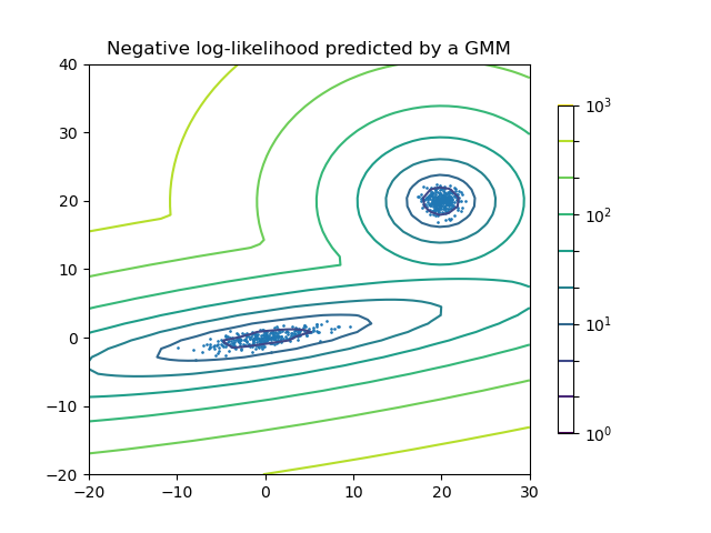
Plot the density estimation of a mixture of two Gaussians. Data is generated from two Gaussians with different centers and covariance matrices.

import numpy as np
import matplotlib.pyplot as plt
from matplotlib.colors import LogNorm
from sklearn import mixture

n_samples = 300

# generate random sample, two components
np.random.seed(0)

# generate spherical data centered on (20, 20)
shifted_gaussian = np.random.randn(n_samples, 2) + np.array([20, 20])

# generate zero centered stretched Gaussian data
C = np.array([[0., -0.7], [3.5, .7]])
stretched_gaussian = np.dot(np.random.randn(n_samples, 2), C)

# concatenate the two datasets into the final training set
X_train = np.vstack([shifted_gaussian, stretched_gaussian])

# fit a Gaussian Mixture Model with two components
clf = mixture.GaussianMixture(n_components=2, covariance_type='full')
clf.fit(X_train)

# display predicted scores by the model as a contour plot
x = np.linspace(-20., 30.)
y = np.linspace(-20., 40.)
X, Y = np.meshgrid(x, y)
XX = np.array([X.ravel(), Y.ravel()]).T
Z = -clf.score_samples(XX)
Z = Z.reshape(X.shape)

CS = plt.contour(X, Y, Z, norm=LogNorm(vmin=1.0, vmax=1000.0),
                 levels=np.logspace(0, 3, 10))
CB = plt.colorbar(CS, shrink=0.8, extend='both')
plt.scatter(X_train[:, 0], X_train[:, 1], .8)

plt.title('Negative log-likelihood predicted by a GMM')
plt.axis('tight')
plt.show()

Total running time of the script: (0 minutes 0.219 seconds)