Non-linear SVM

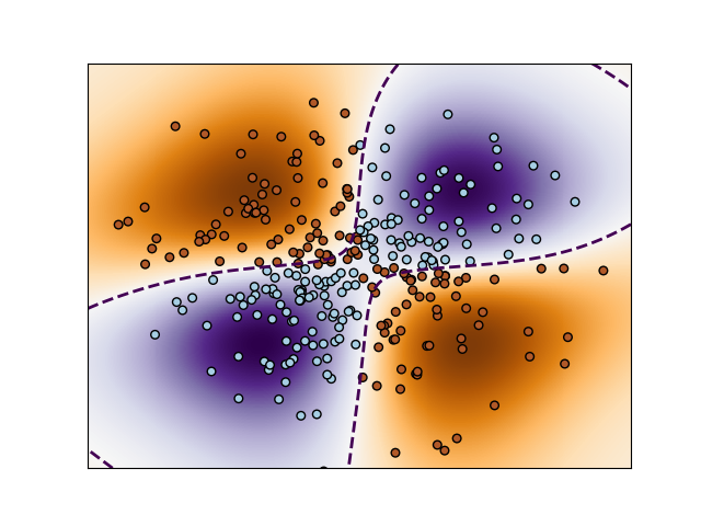
Perform binary classification using non-linear SVC with RBF kernel. The target to predict is a XOR of the inputs.

The color map illustrates the decision function learned by the SVC.

../../_images/sphx_glr_plot_svm_nonlinear_001.png

print(__doc__)
 
import numpy as np
import matplotlib.pyplot as plt
from sklearn import svm
 
xx, yy = np.meshgrid(np.linspace(-3, 3, 500),
                     np.linspace(-3, 3, 500))
np.random.seed(0)
X = np.random.randn(300, 2)
Y = np.logical_xor(X[:, 0] > 0, X[:, 1] > 0)
 
# fit the model
clf = svm.NuSVC()
clf.fit(X, Y)
 
# plot the decision function for each datapoint on the grid
Z = clf.decision_function(np.c_[xx.ravel(), yy.ravel()])
Z = Z.reshape(xx.shape)
 
plt.imshow(Z, interpolation='nearest',
           extent=(xx.min(), xx.max(), yy.min(), yy.max()), aspect='auto',
           origin='lower', cmap=plt.cm.PuOr_r)
contours = plt.contour(xx, yy, Z, levels=[0], linewidths=2,
                       linetypes='--')
plt.scatter(X[:, 0], X[:, 1], s=30, c=Y, cmap=plt.cm.Paired)
plt.xticks(())
plt.yticks(())
plt.axis([-3, 3, -3, 3])
plt.show()

Total running time of the script: (0 minutes 1.229 seconds)

Download Python source code: plot_svm_nonlinear.py

Download IPython notebook: plot_svm_nonlinear.ipynb

Links:

http://scikit-learn.org/stable/auto_examples/svm/plot_svm_nonlinear.html

doc_scikit_learn

2025-01-10 15:47:30

Comments