Comparison of kernel ridge and Gaussian process regression

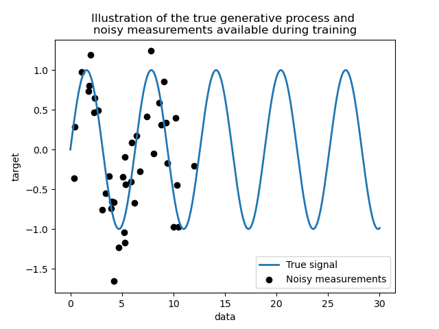
Both kernel ridge regression (KRR) and Gaussian process regression (GPR) learn a target function by employing internally the ?kernel trick?. KRR learns a linear function in the space induced by the respective kernel which corresponds to a non-linear function in the original space. The linear function in the kernel space is chosen based on the mean-squared error loss with ridge regularization. GPR uses the kernel to define the covariance of a prior distribution over the target functions and uses the observed training data to define a likelihood function. Based on Bayes theorem, a (Gaussian) posterior distribution over target functions is defined, whose mean is used for prediction.

A major difference is that GPR can choose the kernel?s hyperparameters based on gradient-ascent on the marginal likelihood function while KRR needs to perform a grid search on a cross-validated loss function (mean-squared error loss). A further difference is that GPR learns a generative, probabilistic model of the target function and can thus provide meaningful confidence intervals and posterior samples along with the predictions while KRR only provides predictions.

This example illustrates both methods on an artificial dataset, which consists of a sinusoidal target function and strong noise. The figure compares the learned model of KRR and GPR based on a ExpSineSquared kernel, which is suited for learning periodic functions. The kernel?s hyperparameters control the smoothness (l) and periodicity of the kernel (p). Moreover, the noise level of the data is learned explicitly by GPR by an additional WhiteKernel component in the kernel and by the regularization parameter alpha of KRR.

The figure shows that both methods learn reasonable models of the target function. GPR correctly identifies the periodicity of the function to be roughly 2*pi (6.28), while KRR chooses the doubled periodicity 4*pi. Besides that, GPR provides reasonable confidence bounds on the prediction which are not available for KRR. A major difference between the two methods is the time required for fitting and predicting: while fitting KRR is fast in principle, the grid-search for hyperparameter optimization scales exponentially with the number of hyperparameters (?curse of dimensionality?). The gradient-based optimization of the parameters in GPR does not suffer from this exponential scaling and is thus considerable faster on this example with 3-dimensional hyperparameter space. The time for predicting is similar; however, generating the variance of the predictive distribution of GPR takes considerable longer than just predicting the mean.

Out:

  Time for KRR fitting: 10.243
Time for GPR fitting: 0.223
Time for KRR prediction: 0.083
Time for GPR prediction: 0.091
Time for GPR prediction with standard-deviation: 0.386

print(__doc__)

# Authors: Jan Hendrik Metzen <jhm@informatik.uni-bremen.de>
# License: BSD 3 clause


import time

import numpy as np

import matplotlib.pyplot as plt

from sklearn.kernel_ridge import KernelRidge
from sklearn.model_selection import GridSearchCV
from sklearn.gaussian_process import GaussianProcessRegressor
from sklearn.gaussian_process.kernels import WhiteKernel, ExpSineSquared

rng = np.random.RandomState(0)

# Generate sample data
X = 15 * rng.rand(100, 1)
y = np.sin(X).ravel()
y += 3 * (0.5 - rng.rand(X.shape[0]))  # add noise

# Fit KernelRidge with parameter selection based on 5-fold cross validation
param_grid = {"alpha": [1e0, 1e-1, 1e-2, 1e-3],
              "kernel": [ExpSineSquared(l, p)
                         for l in np.logspace(-2, 2, 10)
                         for p in np.logspace(0, 2, 10)]}
kr = GridSearchCV(KernelRidge(), cv=5, param_grid=param_grid)
stime = time.time()
kr.fit(X, y)
print("Time for KRR fitting: %.3f" % (time.time() - stime))

gp_kernel = ExpSineSquared(1.0, 5.0, periodicity_bounds=(1e-2, 1e1)) \
    + WhiteKernel(1e-1)
gpr = GaussianProcessRegressor(kernel=gp_kernel)
stime = time.time()
gpr.fit(X, y)
print("Time for GPR fitting: %.3f" % (time.time() - stime))

# Predict using kernel ridge
X_plot = np.linspace(0, 20, 10000)[:, None]
stime = time.time()
y_kr = kr.predict(X_plot)
print("Time for KRR prediction: %.3f" % (time.time() - stime))

# Predict using kernel ridge
stime = time.time()
y_gpr = gpr.predict(X_plot, return_std=False)
print("Time for GPR prediction: %.3f" % (time.time() - stime))

stime = time.time()
y_gpr, y_std = gpr.predict(X_plot, return_std=True)
print("Time for GPR prediction with standard-deviation: %.3f"
      % (time.time() - stime))

# Plot results
plt.figure(figsize=(10, 5))
lw = 2
plt.scatter(X, y, c='k', label='data')
plt.plot(X_plot, np.sin(X_plot), color='navy', lw=lw, label='True')
plt.plot(X_plot, y_kr, color='turquoise', lw=lw,
         label='KRR (%s)' % kr.best_params_)
plt.plot(X_plot, y_gpr, color='darkorange', lw=lw,
         label='GPR (%s)' % gpr.kernel_)
plt.fill_between(X_plot[:, 0], y_gpr - y_std, y_gpr + y_std, color='darkorange',
                 alpha=0.2)
plt.xlabel('data')
plt.ylabel('target')
plt.xlim(0, 20)
plt.ylim(-4, 4)
plt.title('GPR versus Kernel Ridge')
plt.legend(loc="best",  scatterpoints=1, prop={'size': 8})
plt.show()

Total running time of the script: (0 minutes 11.096 seconds)