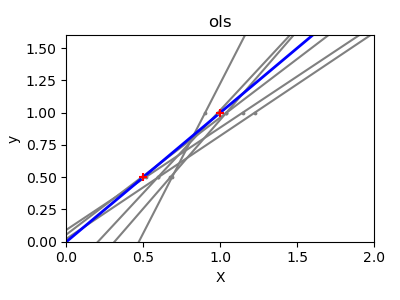
Due to the few points in each dimension and the straight line that linear regression uses to follow these points as well as it can, noise on the observations will cause great variance as shown in the first plot. Every line?s slope can vary quite a bit for each prediction due to the noise induced in the observations.
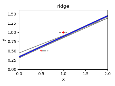
Ridge regression is basically minimizing a penalised version of the least-squared function. The penalising shrinks the value of the regression coefficients. Despite the few data points in each dimension, the slope of the prediction is much more stable and the variance in the line itself is greatly reduced, in comparison to that of the standard linear regression
print(__doc__)


# Code source: Ga Varoquaux
# Modified for documentation by Jaques Grobler
# License: BSD 3 clause


import numpy as np
import matplotlib.pyplot as plt

from sklearn import linear_model

X_train = np.c_[.5, 1].T
y_train = [.5, 1]
X_test = np.c_[0, 2].T

np.random.seed(0)

classifiers = dict(ols=linear_model.LinearRegression(),
                   ridge=linear_model.Ridge(alpha=.1))

fignum = 1
for name, clf in classifiers.items():
    fig = plt.figure(fignum, figsize=(4, 3))
    plt.clf()
    plt.title(name)
    ax = plt.axes([.12, .12, .8, .8])

    for _ in range(6):
        this_X = .1 * np.random.normal(size=(2, 1)) + X_train
        clf.fit(this_X, y_train)

        ax.plot(X_test, clf.predict(X_test), color='.5')
        ax.scatter(this_X, y_train, s=3, c='.5', marker='o', zorder=10)

    clf.fit(X_train, y_train)
    ax.plot(X_test, clf.predict(X_test), linewidth=2, color='blue')
    ax.scatter(X_train, y_train, s=30, c='r', marker='+', zorder=10)

    ax.set_xticks(())
    ax.set_yticks(())
    ax.set_ylim((0, 1.6))
    ax.set_xlabel('X')
    ax.set_ylabel('y')
    ax.set_xlim(0, 2)
    fignum += 1

plt.show()
Total running time of the script: (0 minutes 0.255 seconds)
Download Python source code:
plot_ols_ridge_variance.py
Download IPython notebook:
plot_ols_ridge_variance.ipynb
Please login to continue.