Kernel Density Estimation

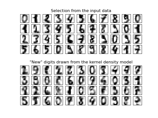
This example shows how kernel density estimation (KDE), a powerful non-parametric density estimation technique, can be used to learn a generative model for a dataset. With this generative model in place, new samples can be drawn. These new samples reflect the underlying model of the data.

../../_images/sphx_glr_plot_digits_kde_sampling_001.png

Out:

1	`best bandwidth:` `3.79269019073`

import numpy as np
import matplotlib.pyplot as plt
 
from sklearn.datasets import load_digits
from sklearn.neighbors import KernelDensity
from sklearn.decomposition import PCA
from sklearn.model_selection import GridSearchCV
 
# load the data
digits = load_digits()
data = digits.data
 
# project the 64-dimensional data to a lower dimension
pca = PCA(n_components=15, whiten=False)
data = pca.fit_transform(digits.data)
 
# use grid search cross-validation to optimize the bandwidth
params = {'bandwidth': np.logspace(-1, 1, 20)}
grid = GridSearchCV(KernelDensity(), params)
grid.fit(data)
 
print("best bandwidth: {0}".format(grid.best_estimator_.bandwidth))
 
# use the best estimator to compute the kernel density estimate
kde = grid.best_estimator_
 
# sample 44 new points from the data
new_data = kde.sample(44, random_state=0)
new_data = pca.inverse_transform(new_data)
 
# turn data into a 4x11 grid
new_data = new_data.reshape((4, 11, -1))
real_data = digits.data[:44].reshape((4, 11, -1))
 
# plot real digits and resampled digits
fig, ax = plt.subplots(9, 11, subplot_kw=dict(xticks=[], yticks=[]))
for j in range(11):
    ax[4, j].set_visible(False)
    for i in range(4):
        im = ax[i, j].imshow(real_data[i, j].reshape((8, 8)),
                             cmap=plt.cm.binary, interpolation='nearest')
        im.set_clim(0, 16)
        im = ax[i + 5, j].imshow(new_data[i, j].reshape((8, 8)),
                                 cmap=plt.cm.binary, interpolation='nearest')
        im.set_clim(0, 16)
 
ax[0, 5].set_title('Selection from the input data')
ax[5, 5].set_title('"New" digits drawn from the kernel density model')
 
plt.show()

Total running time of the script: (0 minutes 15.553 seconds)

Download Python source code: plot_digits_kde_sampling.py

Download IPython notebook: plot_digits_kde_sampling.ipynb

Links:

http://scikit-learn.org/stable/auto_examples/neighbors/plot_digits_kde_sampling.html

doc_scikit_learn

2025-01-10 15:47:30

Comments