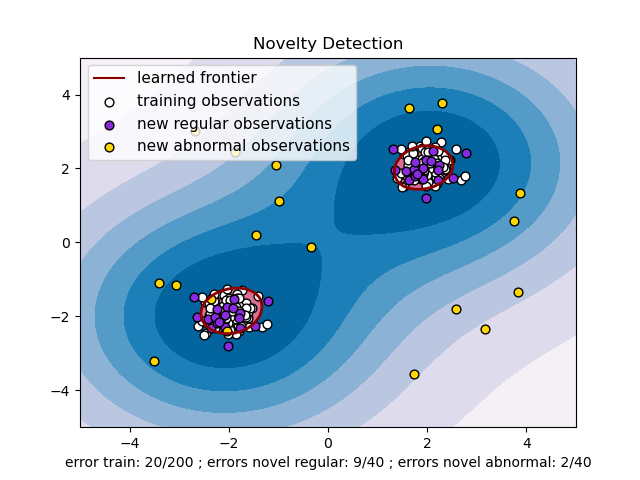
One-class SVM with non-linear kernel

An example using a one-class SVM for novelty detection.

One-class SVM is an unsupervised algorithm that learns a decision function for novelty detection: classifying new data as similar or different to the training set.

../../_images/sphx_glr_plot_oneclass_001.png

print(__doc__)
 
import numpy as np
import matplotlib.pyplot as plt
import matplotlib.font_manager
from sklearn import svm
 
xx, yy = np.meshgrid(np.linspace(-5, 5, 500), np.linspace(-5, 5, 500))
# Generate train data
X = 0.3 * np.random.randn(100, 2)
X_train = np.r_[X + 2, X - 2]
# Generate some regular novel observations
X = 0.3 * np.random.randn(20, 2)
X_test = np.r_[X + 2, X - 2]
# Generate some abnormal novel observations
X_outliers = np.random.uniform(low=-4, high=4, size=(20, 2))
 
# fit the model
clf = svm.OneClassSVM(nu=0.1, kernel="rbf", gamma=0.1)
clf.fit(X_train)
y_pred_train = clf.predict(X_train)
y_pred_test = clf.predict(X_test)
y_pred_outliers = clf.predict(X_outliers)
n_error_train = y_pred_train[y_pred_train == -1].size
n_error_test = y_pred_test[y_pred_test == -1].size
n_error_outliers = y_pred_outliers[y_pred_outliers == 1].size
 
# plot the line, the points, and the nearest vectors to the plane
Z = clf.decision_function(np.c_[xx.ravel(), yy.ravel()])
Z = Z.reshape(xx.shape)
 
plt.title("Novelty Detection")
plt.contourf(xx, yy, Z, levels=np.linspace(Z.min(), 0, 7), cmap=plt.cm.PuBu)
a = plt.contour(xx, yy, Z, levels=[0], linewidths=2, colors='darkred')
plt.contourf(xx, yy, Z, levels=[0, Z.max()], colors='palevioletred')
 
s = 40
b1 = plt.scatter(X_train[:, 0], X_train[:, 1], c='white', s=s)
b2 = plt.scatter(X_test[:, 0], X_test[:, 1], c='blueviolet', s=s)
c = plt.scatter(X_outliers[:, 0], X_outliers[:, 1], c='gold', s=s)
plt.axis('tight')
plt.xlim((-5, 5))
plt.ylim((-5, 5))
plt.legend([a.collections[0], b1, b2, c],
           ["learned frontier", "training observations",
            "new regular observations", "new abnormal observations"],
           loc="upper left",
           prop=matplotlib.font_manager.FontProperties(size=11))
plt.xlabel(
    "error train: %d/200 ; errors novel regular: %d/40 ; "
    "errors novel abnormal: %d/40"
    % (n_error_train, n_error_test, n_error_outliers))
plt.show()

Total running time of the script: (0 minutes 0.286 seconds)

Download Python source code: plot_oneclass.py

Download IPython notebook: plot_oneclass.ipynb

Links:

http://scikit-learn.org/stable/auto_examples/svm/plot_oneclass.html

doc_scikit_learn

2025-01-10 15:47:30

Comments