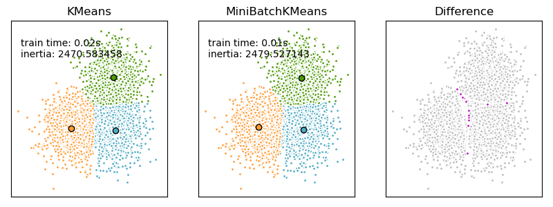
We want to compare the performance of the MiniBatchKMeans and KMeans: the MiniBatchKMeans is faster, but gives slightly different results (see Mini Batch K-Means).
We will cluster a set of data, first with KMeans and then with MiniBatchKMeans, and plot the results. We will also plot the points that are labelled differently between the two algorithms.
print(__doc__)

import time

import numpy as np
import matplotlib.pyplot as plt

from sklearn.cluster import MiniBatchKMeans, KMeans
from sklearn.metrics.pairwise import pairwise_distances_argmin
from sklearn.datasets.samples_generator import make_blobs
Generate sample data
np.random.seed(0)

batch_size = 45
centers = [[1, 1], [-1, -1], [1, -1]]
n_clusters = len(centers)
X, labels_true = make_blobs(n_samples=3000, centers=centers, cluster_std=0.7)
Compute clustering with Means
k_means = KMeans(init='k-means++', n_clusters=3, n_init=10)
t0 = time.time()
k_means.fit(X)
t_batch = time.time() - t0
Compute clustering with MiniBatchKMeans
mbk = MiniBatchKMeans(init='k-means++', n_clusters=3, batch_size=batch_size,
                      n_init=10, max_no_improvement=10, verbose=0)
t0 = time.time()
mbk.fit(X)
t_mini_batch = time.time() - t0
Plot result
fig = plt.figure(figsize=(8, 3))
fig.subplots_adjust(left=0.02, right=0.98, bottom=0.05, top=0.9)
colors = ['#4EACC5', '#FF9C34', '#4E9A06']

# We want to have the same colors for the same cluster from the
# MiniBatchKMeans and the KMeans algorithm. Let's pair the cluster centers per
# closest one.
k_means_cluster_centers = np.sort(k_means.cluster_centers_, axis=0)
mbk_means_cluster_centers = np.sort(mbk.cluster_centers_, axis=0)
k_means_labels = pairwise_distances_argmin(X, k_means_cluster_centers)
mbk_means_labels = pairwise_distances_argmin(X, mbk_means_cluster_centers)
order = pairwise_distances_argmin(k_means_cluster_centers,
                                  mbk_means_cluster_centers)

# KMeans
ax = fig.add_subplot(1, 3, 1)
for k, col in zip(range(n_clusters), colors):
    my_members = k_means_labels == k
    cluster_center = k_means_cluster_centers[k]
    ax.plot(X[my_members, 0], X[my_members, 1], 'w',
            markerfacecolor=col, marker='.')
    ax.plot(cluster_center[0], cluster_center[1], 'o', markerfacecolor=col,
            markeredgecolor='k', markersize=6)
ax.set_title('KMeans')
ax.set_xticks(())
ax.set_yticks(())
plt.text(-3.5, 1.8,  'train time: %.2fs\ninertia: %f' % (
    t_batch, k_means.inertia_))

# MiniBatchKMeans
ax = fig.add_subplot(1, 3, 2)
for k, col in zip(range(n_clusters), colors):
    my_members = mbk_means_labels == order[k]
    cluster_center = mbk_means_cluster_centers[order[k]]
    ax.plot(X[my_members, 0], X[my_members, 1], 'w',
            markerfacecolor=col, marker='.')
    ax.plot(cluster_center[0], cluster_center[1], 'o', markerfacecolor=col,
            markeredgecolor='k', markersize=6)
ax.set_title('MiniBatchKMeans')
ax.set_xticks(())
ax.set_yticks(())
plt.text(-3.5, 1.8, 'train time: %.2fs\ninertia: %f' %
         (t_mini_batch, mbk.inertia_))

# Initialise the different array to all False
different = (mbk_means_labels == 4)
ax = fig.add_subplot(1, 3, 3)

for k in range(n_clusters):
    different += ((k_means_labels == k) != (mbk_means_labels == order[k]))

identic = np.logical_not(different)
ax.plot(X[identic, 0], X[identic, 1], 'w',
        markerfacecolor='#bbbbbb', marker='.')
ax.plot(X[different, 0], X[different, 1], 'w',
        markerfacecolor='m', marker='.')
ax.set_title('Difference')
ax.set_xticks(())
ax.set_yticks(())

plt.show()
Total running time of the script: (0 minutes 0.374 seconds)
Download Python source code:
plot_mini_batch_kmeans.py
Download IPython notebook:
plot_mini_batch_kmeans.ipynb
Please login to continue.